PCoA.py
Create a series of 2D or 3D PCoA plots where the marker size varies by relative abundance of a particular OTU.
usage: PCoA.py [-h] -i COORD_FP -m MAP_FP -b COLORBY [-o OUT_FN] [-d {2,3}][-t TITLE] [--save] [-c MAP_CATEGORIES] [-s POINT_SIZE]
Required Arguments
-
-iCOORD_FP,--coord_fpCOORD_FP¶ Path to the principal coordinates result file (i.e., output from principal_coordinates.py).
-
-mMAP_FP,--map_fpMAP_FP¶ Path to the metadata mapping file.
-
-gGROUP_BY,--group_byGROUP_BY¶ Metadata category/categories (column headers) to group samples by in the plot. A single category can be specified as follows:
-b Treatment. Multiple categories can also be specified:-b Treatment,Age. Finally, each specified category can be fixed to a single value:-b Treatment,Age,Gender=male. Note that in all cased, no spaces should be used). The program will create one group for each unique combination of values for the specified categories and put each sample in the appropriate group that matches its metadata. For example, if Treatment has two values (TreatmentA, TreatmentB) and Gender has two values (male, female), there are a total of 4 possible groups: TreatmentA and male, TreatmentA and female, TreatmentB and male, TreatmentB and female. In the output plot legend, multiple-category groups will have their values joined by an underscore: TreatmentA_male, TreatmentB_female.
Optional Arguments
-
-d{2,3},--dimensions{2,3}¶ Choose whether to plot 2D or 3D. Default is a 2D plot.
-
-cCOLORS,--colorsCOLORS¶ A column name in the mapping file containing hexadecimal (#FF0000) color values that will be used to color the groups. Each sample ID must have a color entry.
-
-sPOINT_SIZE,--point_sizePOINT_SIZE¶ Specify the size of the circles representing each of the samples in the plot.
-
--pc_orderPC_ORDER¶ Choose which Principle Coordinates are displayed and in which order, for example: 1,2 (Note the lack of any spaces around the comma).
-
--x_limitsX_LIMITS X_LIMITS¶ Specify limits for the x-axis instead of automatic setting based on the data range. Should take the form: –x_limits -0.5 0.5
-
--y_limitsY_LIMITS Y_LIMITS¶ Specify limits for the y-axis instead of automatic setting based on the data range. Should take the form: –y_limits -0.5 0.5
-
--z_limitsZ_LIMITS Z_LIMITS¶ Specify limits for the z-axis instead of automatic setting based on the data range. Should take the form: –z_limits -0.5 0.5
-
--z_anglesZ_ANGLES Z_ANGLES¶ Specify the azimuth and elevation angles for a 3D plot.
-
-tTITLE,--titleTITLE¶ Title of the plot.
-
--figsizeFIGSIZE FIGSIZE¶ Specify the ‘width height’ in inches for PCoA plots.By default, figure size is 14x8 inches
-
--font_sizeFONT_SIZE¶ Sets the font size for text elements in the plot.
-
--label_paddingLABEL_PADDING¶ Sets the spacing in points between the each axis and its label.
-
--annotate_points¶ If specified, each graphed point will be labeled with its sample ID.
-
--ggplot2_style¶ Apply ggplot2 styling to the figure.
-
-oOUT_FP,--out_fpOUT_FP¶ The path and file name to save the plot under. If specified, the figure will be saved directly instead of opening a window in which the plot can be viewed before saving.
-
-h,--help¶ Show the help message and exit.
Workflow for generating PCoA plots using PhyloToAST
Step 1 : Create an all-pairs distance matrix for your sample data using the beta_diversity.py QIIME script. Different distance metrics can be calculated here: bray_cutis, morisita_horn, kulczynski, and many others.
Step 2 : Perform a principal coordinates analysis of the distance matrix from Step 1 using QIIME’s principal_coordinates.py script.
Alternate Step 1 and 2 combined for UniFrac PCoA: The beta_diversity_through_plots.py script produces the PCoA analysis of the UniFrac distances (weighted and unweighted) in one step.
Step 3 :
Run PhyloToAST’s PCoA.py with the input (-i) set to the output from Step 2.
For minimum functionality, also set the mapping file (-m), and the grouping category column
within the mapping file (-b). If you want to specify your own colors for the groups, also specify
-c option. To get a 3D plot that is rotatable/zoomable specify -d 3.
Example plots
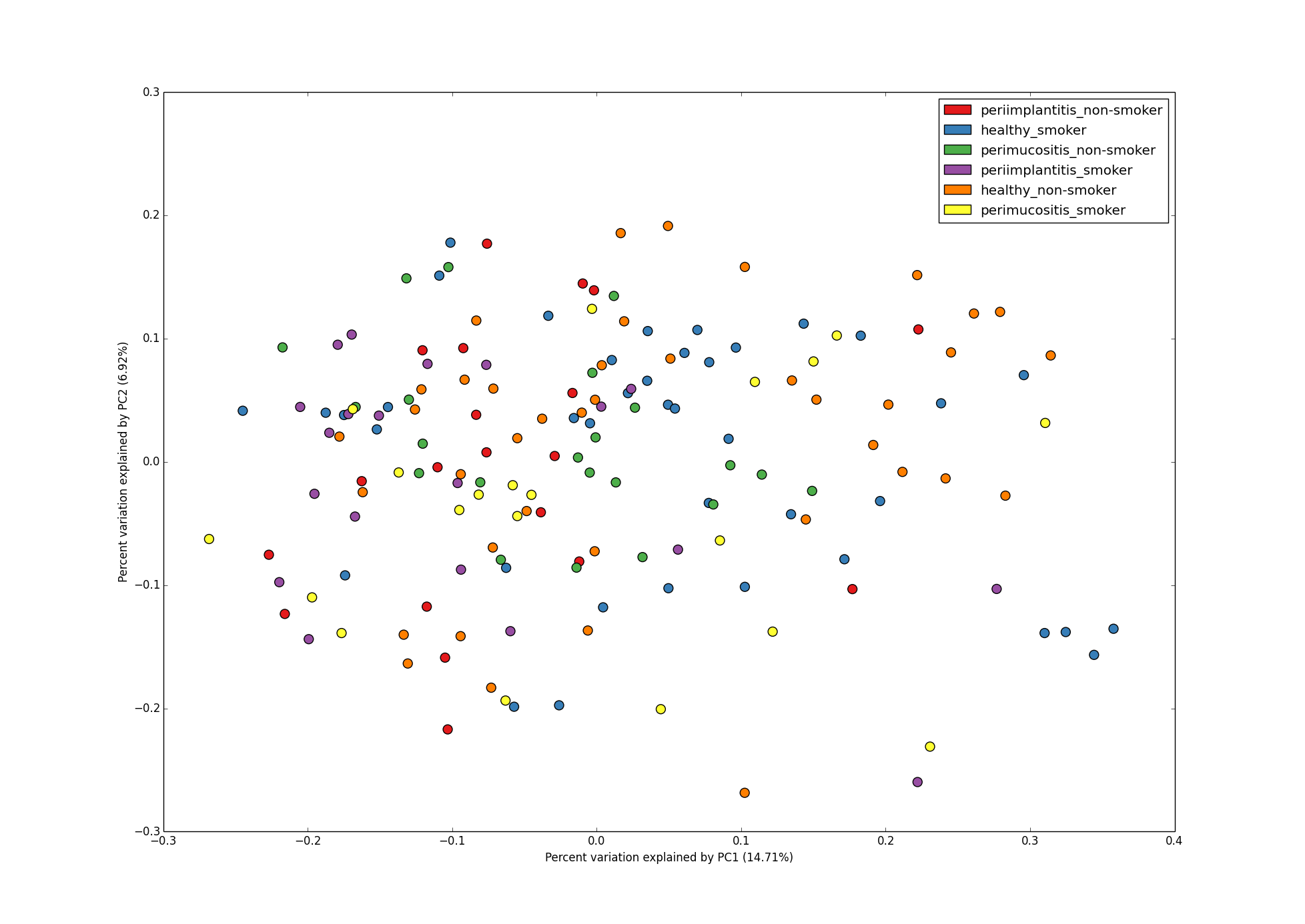
2D PCoA plot with 2 metadata categories - DiseaseState and SmokingStatus.
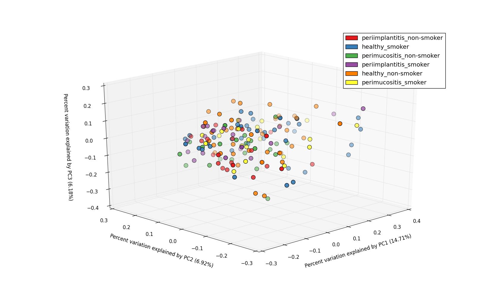
3D PCoA plot with 2 metadata categories - DiseaseState and SmokingStatus.